1. Introduction to MCW testing
Originally, Monte Carlo-Wilcoxon (MCW) tests were designed to determined whether the differences between two sets of data were significantly biased in the same direction when compared with what it would be expected by chance. MCW tests proceed by calculating sum-of-ranks-based bias indexes, hence the reference to Frank Wilcoxon who invented the non-parametric rank-sum and signed-rank tests, before and after rearranging the dataset multiple times, hence the Monte Carlo reference often associated to analytical strategies based on repeated random sampling1–5.
The MCWtests package encompasses the original MCW test and three variations that differ in the data structures and the specific questions they interrogate.
The matched-measures univariate MCW (muMCW) test, the original MCW test1–5, assesses whether one set of inherently matched-paired measures is significantly biased in the same direction. For instance, muMCW tests can be used to analyze bodyweights or transcript abundances determined at two different timepoints for the same set of mice.
The unmatched-measures MCW (uMCW) test assesses whether two sets of unmatched measures and their heterogeneity are significantly biased in the same direction. For instance, uMCW tests can be used to analyze bodyweights or transcript abundances determined for two sets of mice that have been maintained in different conditions.
The matched-measures bivariate MCW (mbMCW) test assesses whether two sets of inherently matched-paired measures are significantly differentially biased in the same direction. For instance, mbMCW tests can be used to analyze bodyweights or transcript abundances determined at two different timepoints for two sets of mice that have been exposed to different conditions.
The bias-measures MCW (bMCW) test assesses whether a set of measures of bias for a quantitative trait between two conditions or a subset of these bias measures are themselves significantly biased in the same direction. For instance, bMCW tests can be used to analyze bias indexes obtained using other MCW tests or fold change for transcript abundances spanning the entire transcriptome or only for genes located in specific genomic regions from two sets of mice exposed to different conditions.
2. MCW testing process
Although each MCW test examines distinct data structures to address slightly different questions, all MCW tests share two fundamental steps:
To quantitatively determine the extent and direction of the bias of the measure under analysis, MCW tests calculate a bias index (BI) by summing ranks and dividing these sums by the maximum possible value of the sums. Consequently, BIs range from 1 to -1 when the measure under analysis is completely biased in each possible direction.
To determine the significance of the BIs calculated for the user-provided dataset (observed BIs), a collection of expected-by-chance BIs is generated by rearranging the original dataset multiple times and calculating BIs for each iteration. Pupper and Plower values are calculated as the fractions of expected-by-chance BIs that have values higher or equal to and lower or equal to the observed BIs, respectively.
Each MCW test employs the user-provided parameter max_rearrangements to follow two alternative paths.
MCW exact tests. If the number of distinct rearrangements that can be generated from the dataset under analysis is less than max_rearrangements, MCW tests will actually generate all possible data rearrangements to create the collection of expected-by-chance BIs. In this case, Pupper and Plower values will be exact estimations of the likelihood of obtaining BIs with equal or more extreme values compared to observed BIs with datasets of the same size and range but different internal structures.
MCW approximated tests. If the number of distinct rearrangements that can be generated from the dataset under analysis is greater than max_rearrangements, MCW tests will perform a specified number of random data rearrangements, equal to the value of max_rearrangements, to generate the collection of expected-by-chance BIs. In this case, Pupper and Plower values will represent approximate estimations of the likelihood of obtaining BIs with equal or more extreme values compared to observed BIs with datasets of the same size and range but different internal structures.
3. MCWtests data and function structure
Each MCW test involves two local files, one exported function that users interacts with, and several internal functions that perform specific tasks.
- Local files:
Entry CSV dataset. Users provide data for MCW testing in a CSV file in the directory of their choice. This file can contain data for a single MCW test or multiple MCW tests to be executed simultaneously. Users can organize the entry dataset in two different layouts, vertical or horizontal, which is particularly useful for simultaneous testing when the data structures for each individual test are significantly different or very similar, respectively.
Results CSV table. MCW test functions create a CSV file with the results of MCW testing, with a similar name to the entry CSV dataset file, in the same directory where the entry CSV is located.
- Exported functions:
-
MCWtest function: When executing this function, users must specify the path to the CSV file containing the entry dataset and the parameter max_rearrangements. The MCWtest function interprets this parameter as the maximum number of data rearrangement iterations used to define the size of the collection of expected-by-chance BIs. The MCWtest function performs the following tasks:
- It loads the entry CSV dataset.
- It determines whether MCW tests will proceed using the exact or approximated testing paths.
- It calls the corresponding functions, MCW_exact_test and MCW_approximated_test, to run the exact and approximated tests, resepctively.
- It writes the results of MCW testing to a CSV file in the same directory as the entry CSV file.
- Internal functions:
-
MCW_exact_test function: This function is called when the number of distinctive data rearrangements is less than the user-provided parameter max_rearrangements. The MCW_exact_test function performs the following tasks:
- It generates all distinctive data rearrangements, either on its own or by executing the MCW_exact_test_combinations function.
- It calculates BIs for the user-provided data and each of the distinctive rearrangements of the dataset.
- It calculates the Pupper and Plower values as the fractions of expected-by-chance BIs with values higher or equal to and lower or equal to the observed BIs, respectively.
- It returns the MCW exact testing results to the MCWtest function.
MCW_exact_test_combinations function: This function is called to assist the MCW_exact_test function in generating all distinctive data rearrangements.
-
MCW_approximated_test function: This function is called when the number of distinctive data rearrangements is greater than the user-provided parameter max_rearrangements. The MCW_approximated_test function performs the following tasks:
- It calls the MCW_approximated_test_observed_BIs function to calculate BIs for the user-provided dataset.
- It calls the MCW_approximated_test_simulated_BIs function to randomly rearrange the data and calculate the expected-by-chance BIs a specified number of times, which is equal to max_rearrangements.
- It calculates the Pupper and Plower values as the fractions of expected-by-chance BIs with values higher or equal to and lower or equal to the observed BIs, respectively.
- It returns the MCW approximated testing results to the MCWtest function
MCW_approximated_test_observed_BIs function: This function is called to calculate BIs for the user-provided dataset.
MCW_approximated_test_simulated_BIs function: This function is called N times, where N = max_rearrangements, to randomly rearrange the data and calculate the expected-by-chance BIs using the MCW_approximated_test_observed_BIs function.
4. Specific MCW tests
4.1 unmatched-measures MCW (uMCW) test
Introduction
The uMCW test is actually a combination of two different tests that assess whether two sets of unmatched measures and their heterogeneity are significantly biased in the same direction. Significantly different data heterogeneities between two conditions could indicate that the measure under analysis is more constrained or more relaxed in one of the conditions, potentially providing insights into the mechanisms underlying the variation of such measure. For instance, uMCW tests can be used to analyze bodyweights or transcript abundances determined for two sets of mice that have been maintained in different conditions.
uMCW testing entry dataset formatting
When executing the uMCWtest function, users must provide the path to a local CSV file named X_uMCWtest_data.csv, where X serves as a user-defined identifier. X_uMCWtest_data.csv can be structured in two distinct formats:
-
Vertical layout: This format allows appending datasets with varying structures, such as different numbers of measures per set or between each appended test. Vertical entry datasets should include the following columns:
- The condition column uniquely identifies each of the two measure sets under analysis.
- The value column contains the actual measures under analysis.
- As many informative columns as needed by users to contextualize the results of each test. The names of these columns should not include the terms condition or value. While these columns are optional when running a single test, at least one column is required when running multiple tests simultaneously. All rows for each individual test must contain the same information in these columns.
-
Horizontal layout: This format allows appending datasets with similar structures, such as the same number of measures collected for each of the two conditions. Horizontal entry datasets should include the following columns:
- Columns condition_a and condition_b uniquely identify the two measure sets under analysis.
- Columns a.i and b.j, where i and j represent integers to differentiate specific measures within each set, contain the actual measures under analysis.
- As many informative columns as needed by users to contextualize the results of each test. The names of these columns should not contain the term condition or have the same structure as the a.i and b.j columns. While these columns are optional when running a single test, at least one column is required when running multiple tests simultaneously.
uMCW testing process
The function uMCWtest eliminate missing values (NAs) from the dataset before proceeding these steps.
-
To estimate the bias between the two sets of measures (e.g., a and b), the function uMCWtest performs these tasks:
- It generates all possible disjoint data pairs using measures from both sets.
- For each measure pair, it subtracts the second measure in the pair from the first measure in the pair.
- It ranks the absolute values of all non-zero measure pair differences from lowest to highest. Measure pair differences with a value of 0 are assigned a 0 rank. If multiple measure pair differences have the same absolute value, all tied measure pair differences are assigned the lowest rank possible.
- It assigns each measure pair rank a sign based on the sign of its corresponding measure pair difference.
- It sums the signed ranks for measure pairs formed with measures from the two different sets (e.g., a-b and b-a).
- For each type of disjoint set measure pairs (e.g., a-b and b-a), it calculates uMCW_BI by dividing the sum of signed ranks by the maximum number this sum could have if the corresponding measure pairs had the highest possible positive ranks. Consequently, uMCW_BI ranges between 1 when all the values for measures in the first set are higher than all the values from measures in the second set, and -1 when all the values for measures in the first set are lower than all the values from measures in the second set.
-
To estimate the bias between the heterogeneity of two sets of measures, the function uMCWtest performs these tasks:
- It generates all possible disjoint data pairs within each set, disregarding the order of the paired measures. For instance, the measure pair a.1-a.2 is considered equivalent to the measure pair a.2-a.1, and only the former is retained for the subsequent calculations.
- For each measure pair, it subtracts the second measure from the first measure.
- It ranks all measure pair differences with non-zero values from lowest to highest. Measure pair differences with a value of 0 are assigned a 0 rank. If multiple measure pair differences have the same absolute value, uMCWtest assigns all tied measure pair differences the lowest rank possible.
- It sums ranks for measure pairs formed with measures from the same set (e.g., a-a and b-b).
- For each type of same-set measure pairs (e.g., a-a and b-b), it divides each sum of signed ranks by the maximum number this sum could have if the corresponding measure pairs had the highest possible ranks.
- It calculates two heterogeneity bias indexes (uMCW_HBIs) by subtracting the normalized sum of signed ranks from the previous step in two possible directions (e.g., a-b and b-a). Consequently, uMCW_HBI ranges between 1 when at least two measures in the first set have distinct values and all measures in the second set have the same value, and -1 when all measures in the first set have the same value and at least two measures in the second set have distinct values.
-
To assess the significance of the uMCW_BIs and uMCW_HBIs obtained with the user-provided data (observed uMCW_BIs and uMCW_HBIs), the function uMCWtest performs these tasks:
-
It generates a collection of expected-by-chance uMCW_BIs and uMCW_HBIs. These expected values are obtained by rearranging the measures between the two sets multiple times. The user-provided parameter max_rearrangements determines the two paths that the function uMCWtest can follow to generate the collection of expected-by-chance uMCW_BIs and uMCW_HBIs:
- uMCW exact testing: If the number of distinct measure rearrangements that can alter their initial set distribution is less than max_rearrangements, the function uMCWtest calculates uMCW_BIs and uMCW_HBIs for all possible data rearrangements.
- uMCW approximated testing: If the number of distinct measure rearrangements that can alter their initial set distribution is greater than max_rearrangements, the function uMCWtest will perform N = max_rearrangements random measure rearrangements to calculate the collection of expected-by-chance uMCW_BIs and uMCW_HBIs.
It calculates Pupper and Plower values as the fraction of expected-by-chance uMCW_BIs and uMCW_HBIs that are higher or equal to and lower or equal to the observed uMCW_BIs and uMCW_HBIs, respectively.
-
uMCW testing results
The uMCWtest function reports to the console the total number of tests it will execute, and their exact and approximated counts. It also creates a CSV file named X_uMCWtest_results.csv, where X is a user-defined identifier for the entry dataset CSV file. The X_uMCWtest_results.csv file contains four rows for each uMCWtest, two for uMCW_BIs calculated for each condition contrast (e.g., a-b and b-a), and two for uMCW_HBIs calculated for each condition contrast.
The X_uMCWtest_results.csv file includes the following columns:
- User-provided informative columns to contextualize the results of each test.
- Columns condition_a and condition_b indicate the two measure sets under analysis.
- Columns N, n_a and n_b indicate the total number of measures and the number of measures belonging to each set after removing missing values (NAs).
- Column test_type distinguishes between exact and approximated tests.
- Column BI_type indicates the bias index type (uMCW_BI and uMCW_HBI) for each row of results.
- Column condition_contrast indicates the set contrast (e.g., a-b or b-a) for each row of results.
- Column observed_BI contains the values of uMCW_BIs and uMCW_HBIs obtained from analyzing the user-provided dataset.
- Column expected_by_chance_BI_N indicates the number of data rearrangements used to calculate the expected-by-chance uMCW_BIs and uMCW_HBIs. This value corresponds to the lowest number between all possible measure rearrangements and the parameter max_rearrangements.
- Columns pupper and plower represent the Pupper and Plower values, respectively. They denote the fraction of expected-by-chance uMCW_BIs or uMCW_HBIs with values higher or equal to and lower or equal to the observed uMCW_BIs or uMCW_HBIs, respectively.
Examples
uMCW testing of multiple datasets organized vertically
This example of uMCW testing entry dataset with a vertical layout showcases data for three ideal tests (Table 1). The Contrast I test includes data for two sets of measures randomly selected from the same range (Figure 1). The Contrast II test includes data representing two sets of measures randomly selected from two different ranges, with measures from the second set being generally higher than those from the first set (Figure 1). The Contrast III test includes data representing two sets of measures randomly selected from two different ranges, with measures from the second set being generally higher and less heterogeneous than those from the first set (Figure 1). The results of these uMCW tests align with the intended structure of the entry datasets (Table 2).
Table 1. uMCW testing entry dataset with vertical layout
    contrast condition value
      <char>    <char> <int>
 1:        I      AAAA    63
 2:        I      AAAA    22
 3:        I      AAAA    87
 4:        I      AAAA    34
 5:        I      AAAA    27
 6:        I      BBBB    32
 7:        I      BBBB    10
 8:        I      BBBB    74
 9:        I      BBBB    31
10:        I      BBBB    76
11:       II      AAAA    51
12:       II      AAAA     5
13:       II      AAAA    25
14:       II      AAAA     4
15:       II      AAAA    38
16:       II      BBBB    68
17:       II      BBBB    98
18:       II      BBBB    41
19:       II      BBBB   100
20:       II      BBBB    67
21:      III      AAAA    46
22:      III      AAAA    14
23:      III      AAAA    35
24:      III      AAAA    11
25:      III      AAAA    36
26:      III      BBBB    56
27:      III      BBBB    51
28:      III      BBBB    50
29:      III      BBBB    51
30:      III      BBBB    60
    contrast condition value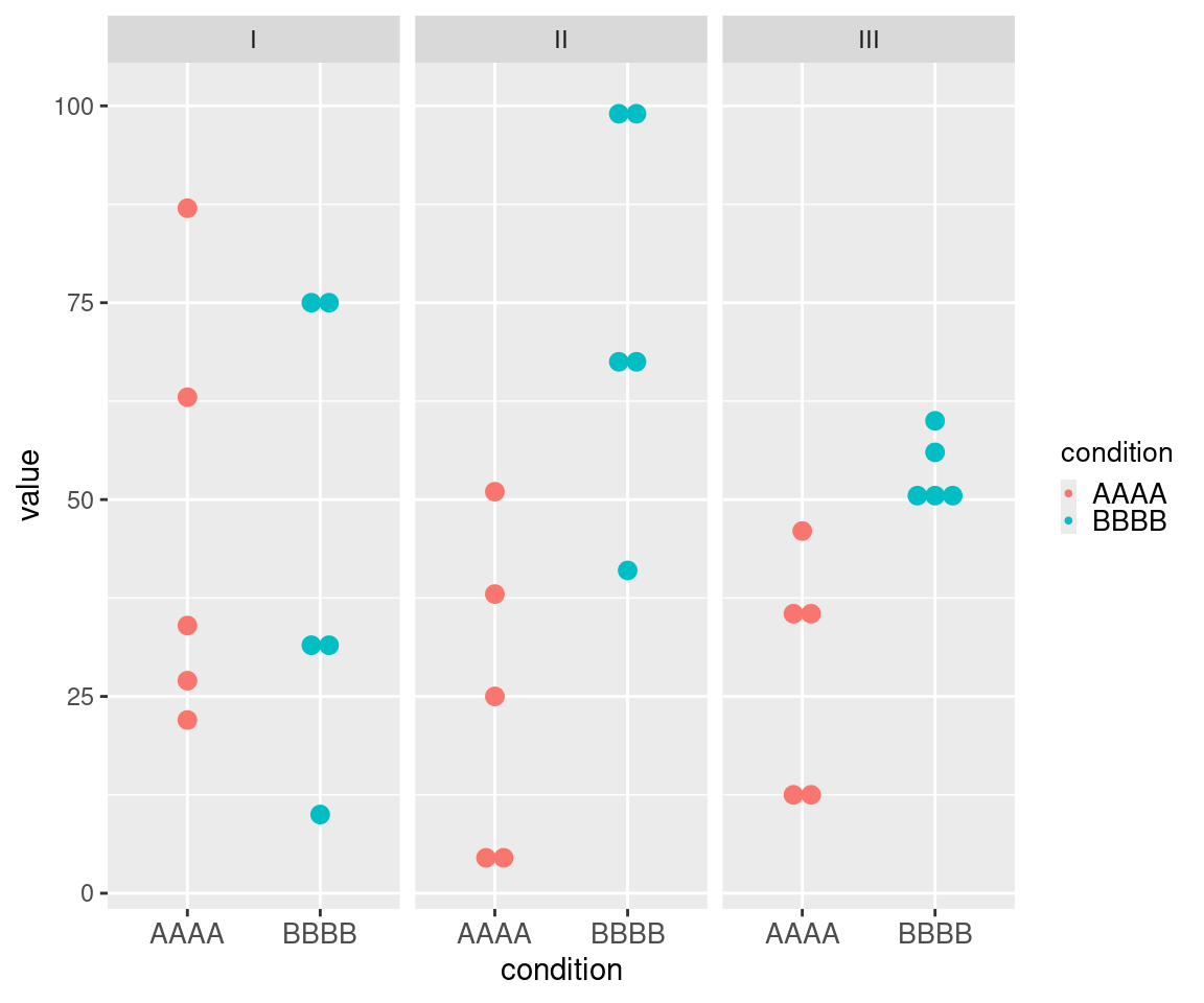
Table 2. Results of uMCW testing using an entry dataset with vertical layout
    contrast condition_a condition_b     N   n_a   n_b    test_type  BI_type
      <char>      <char>      <char> <int> <int> <int>       <char>   <char>
 1:        I        AAAA        BBBB    10     5     5 approximated  uMCW_BI
 2:        I        AAAA        BBBB    10     5     5 approximated  uMCW_BI
 3:        I        AAAA        BBBB    10     5     5 approximated uMCW_HBI
 4:        I        AAAA        BBBB    10     5     5 approximated uMCW_HBI
 5:       II        AAAA        BBBB    10     5     5 approximated  uMCW_BI
 6:       II        AAAA        BBBB    10     5     5 approximated  uMCW_BI
 7:       II        AAAA        BBBB    10     5     5 approximated uMCW_HBI
 8:       II        AAAA        BBBB    10     5     5 approximated uMCW_HBI
 9:      III        AAAA        BBBB    10     5     5 approximated  uMCW_BI
10:      III        AAAA        BBBB    10     5     5 approximated  uMCW_BI
11:      III        AAAA        BBBB    10     5     5 approximated uMCW_HBI
12:      III        AAAA        BBBB    10     5     5 approximated uMCW_HBI
    condition_contrast observed_BI expected_by_chance_BI_N pupper plower
                <char>       <num>                   <int>  <num>  <num>
 1:          AAAA-BBBB  0.03948718                     200  0.430  0.595
 2:          BBBB-AAAA -0.03948718                     200  0.595  0.430
 3:          AAAA-BBBB -0.02857143                     200  0.500  0.505
 4:          BBBB-AAAA  0.02857143                     200  0.505  0.500
 5:          AAAA-BBBB -0.69794872                     200  1.000  0.005
 6:          BBBB-AAAA  0.69794872                     200  0.005  1.000
 7:          AAAA-BBBB -0.07766990                     200  0.720  0.285
 8:          BBBB-AAAA  0.07766990                     200  0.285  0.720
 9:          AAAA-BBBB -0.68358974                     200  1.000  0.000
10:          BBBB-AAAA  0.68358974                     200  0.000  1.000
11:          AAAA-BBBB  0.39130435                     200  0.040  0.970
12:          BBBB-AAAA -0.39130435                     200  0.970  0.040
uMCW testing of multiple datasets organized horizontally
This example of uMCW testing entry dataset with a horizontal layout showcases data for nine ideal tests (Table 3). It includes two types of informative columns to accommodate cases where users might want to perform multiple tests with a nested structure. The columns with the contrast prefix provide contextual information for groups of tests or rows, while the columns with the element prefix provide contextual information for each test or row. Each Contrast I row includes two sets of measures randomly selected from the same range (Figure 2). Each Contrast II row includes two sets of measures randomly selected from two different ranges, with the measures from the second set being generally higher than those from the first set (Figure 2). Each Contrast III row includes two sets of measures randomly selected from two different ranges, with the measures from the second set being generally higher and less heterogeneous than those from the first set (Figure 1). The results of these uMCW tests align with the intended structure of the entry datasets (Table 4).
Table 3. uMCW testing entry dataset with horizontal layout
   contrast contrast_trait element_ID element_chr element_start element_end
     <char>         <char>     <char>       <int>         <int>       <int>
1:        I        trait_a         x1           1          1000        2000
2:        I        trait_a         x2           1          5000        5500
3:        I        trait_a         x3           1         90000      100000
4:       II        trait_b         x1           1          1000        2000
5:       II        trait_b         x2           1          5000        5500
6:       II        trait_b         x3           1         90000      100000
7:      III        trait_b         x1           1          1000        2000
8:      III        trait_b         x2           1          5000        5500
9:      III        trait_b         x3           1         90000      100000
   condition_a condition_b   a.1   a.2   a.3   a.4   a.5   b.1   b.2   b.3
        <char>      <char> <int> <int> <int> <int> <int> <int> <int> <int>
1:        AAAA        BBBB    91    56    65    63    23    17    NA    50
2:        AAAA        BBBB    96    45    42    29    12    25    36    28
3:        AAAA        BBBB    77    98    31    93    34    34    97    77
4:        AAAA        BBBB    54    23    59    28    52    90    92    91
5:        AAAA        BBBB    37     5    18    26    11    48    84    62
6:        AAAA        BBBB    28    35    43    13     6    60    71    77
7:        AAAA        BBBB    20    32    14     3     6    46    56    45
8:        AAAA        BBBB    50    38    28    47    27    55    46    51
9:        AAAA        BBBB    31    36     2    37    47    54    48    48
     b.4   b.5
   <int> <int>
1:    39    30
2:    79    82
3:    53    11
4:    50    68
5:    86    53
6:    89    97
7:    57    50
8:    46    60
9:    46    48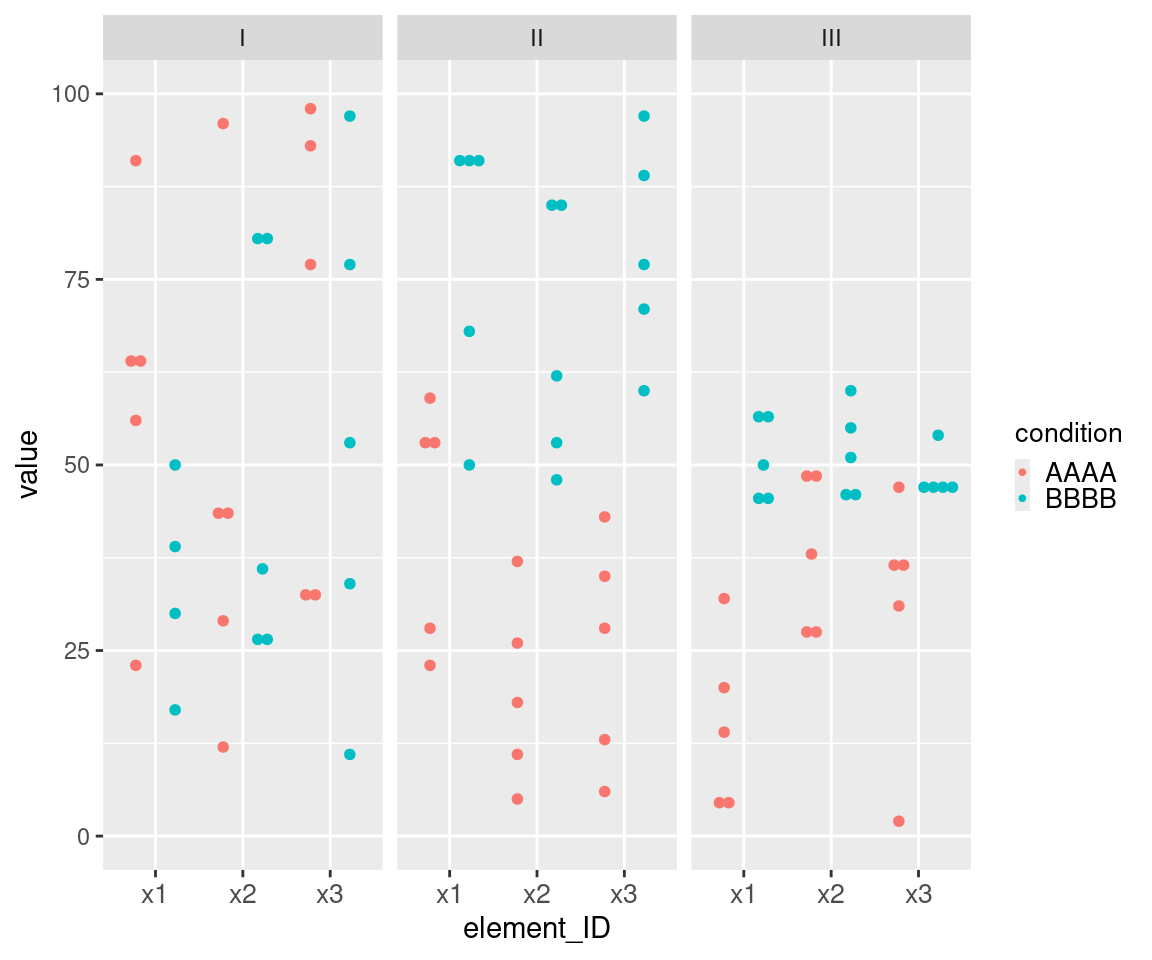
Table 4. Results of uMCW testing using an entry dataset with horizontal layout
    contrast contrast_trait element_ID element_chr element_start element_end
      <char>         <char>     <char>       <int>         <int>       <int>
 1:        I        trait_a         x1           1          1000        2000
 2:        I        trait_a         x1           1          1000        2000
 3:        I        trait_a         x1           1          1000        2000
 4:        I        trait_a         x1           1          1000        2000
 5:        I        trait_a         x2           1          5000        5500
 6:        I        trait_a         x2           1          5000        5500
 7:        I        trait_a         x2           1          5000        5500
 8:        I        trait_a         x2           1          5000        5500
 9:        I        trait_a         x3           1         90000      100000
10:        I        trait_a         x3           1         90000      100000
11:        I        trait_a         x3           1         90000      100000
12:        I        trait_a         x3           1         90000      100000
13:       II        trait_b         x1           1          1000        2000
14:       II        trait_b         x1           1          1000        2000
15:       II        trait_b         x1           1          1000        2000
16:       II        trait_b         x1           1          1000        2000
17:       II        trait_b         x2           1          5000        5500
18:       II        trait_b         x2           1          5000        5500
19:       II        trait_b         x2           1          5000        5500
20:       II        trait_b         x2           1          5000        5500
21:       II        trait_b         x3           1         90000      100000
22:       II        trait_b         x3           1         90000      100000
23:       II        trait_b         x3           1         90000      100000
24:       II        trait_b         x3           1         90000      100000
25:      III        trait_b         x1           1          1000        2000
26:      III        trait_b         x1           1          1000        2000
27:      III        trait_b         x1           1          1000        2000
28:      III        trait_b         x1           1          1000        2000
29:      III        trait_b         x2           1          5000        5500
30:      III        trait_b         x2           1          5000        5500
31:      III        trait_b         x2           1          5000        5500
32:      III        trait_b         x2           1          5000        5500
33:      III        trait_b         x3           1         90000      100000
34:      III        trait_b         x3           1         90000      100000
35:      III        trait_b         x3           1         90000      100000
36:      III        trait_b         x3           1         90000      100000
    contrast contrast_trait element_ID element_chr element_start element_end
    condition_a condition_b     N   n_a   n_b    test_type  BI_type
         <char>      <char> <int> <int> <int>       <char>   <char>
 1:        AAAA        BBBB     9     5     4        exact  uMCW_BI
 2:        AAAA        BBBB     9     5     4        exact uMCW_HBI
 3:        AAAA        BBBB     9     5     4        exact  uMCW_BI
 4:        AAAA        BBBB     9     5     4        exact uMCW_HBI
 5:        AAAA        BBBB    10     5     5 approximated  uMCW_BI
 6:        AAAA        BBBB    10     5     5 approximated  uMCW_BI
 7:        AAAA        BBBB    10     5     5 approximated uMCW_HBI
 8:        AAAA        BBBB    10     5     5 approximated uMCW_HBI
 9:        AAAA        BBBB    10     5     5 approximated  uMCW_BI
10:        AAAA        BBBB    10     5     5 approximated  uMCW_BI
11:        AAAA        BBBB    10     5     5 approximated uMCW_HBI
12:        AAAA        BBBB    10     5     5 approximated uMCW_HBI
13:        AAAA        BBBB    10     5     5 approximated  uMCW_BI
14:        AAAA        BBBB    10     5     5 approximated  uMCW_BI
15:        AAAA        BBBB    10     5     5 approximated uMCW_HBI
16:        AAAA        BBBB    10     5     5 approximated uMCW_HBI
17:        AAAA        BBBB    10     5     5 approximated  uMCW_BI
18:        AAAA        BBBB    10     5     5 approximated  uMCW_BI
19:        AAAA        BBBB    10     5     5 approximated uMCW_HBI
20:        AAAA        BBBB    10     5     5 approximated uMCW_HBI
21:        AAAA        BBBB    10     5     5 approximated  uMCW_BI
22:        AAAA        BBBB    10     5     5 approximated  uMCW_BI
23:        AAAA        BBBB    10     5     5 approximated uMCW_HBI
24:        AAAA        BBBB    10     5     5 approximated uMCW_HBI
25:        AAAA        BBBB    10     5     5 approximated  uMCW_BI
26:        AAAA        BBBB    10     5     5 approximated  uMCW_BI
27:        AAAA        BBBB    10     5     5 approximated uMCW_HBI
28:        AAAA        BBBB    10     5     5 approximated uMCW_HBI
29:        AAAA        BBBB    10     5     5 approximated  uMCW_BI
30:        AAAA        BBBB    10     5     5 approximated  uMCW_BI
31:        AAAA        BBBB    10     5     5 approximated uMCW_HBI
32:        AAAA        BBBB    10     5     5 approximated uMCW_HBI
33:        AAAA        BBBB    10     5     5 approximated  uMCW_BI
34:        AAAA        BBBB    10     5     5 approximated  uMCW_BI
35:        AAAA        BBBB    10     5     5 approximated uMCW_HBI
36:        AAAA        BBBB    10     5     5 approximated uMCW_HBI
    condition_a condition_b     N   n_a   n_b    test_type  BI_type
    condition_contrast  observed_BI expected_by_chance_BI_N     pupper
                <char>        <num>                   <int>      <num>
 1:          AAAA-BBBB  0.500800000                     126 0.06349206
 2:          AAAA-BBBB  0.402985075                     126 0.25396825
 3:          BBBB-AAAA -0.500800000                     126 0.94444444
 4:          BBBB-AAAA -0.402985075                     126 0.76984127
 5:          AAAA-BBBB -0.066153846                     200 0.58000000
 6:          BBBB-AAAA  0.066153846                     200 0.42500000
 7:          AAAA-BBBB  0.064039409                     200 0.41000000
 8:          BBBB-AAAA -0.064039409                     200 0.59500000
 9:          AAAA-BBBB  0.161538462                     200 0.31500000
10:          BBBB-AAAA -0.161538462                     200 0.70500000
11:          AAAA-BBBB -0.043062201                     200 0.54500000
12:          BBBB-AAAA  0.043062201                     200 0.47000000
13:          AAAA-BBBB -0.649743590                     200 0.98000000
14:          BBBB-AAAA  0.649743590                     200 0.02000000
15:          AAAA-BBBB  0.024390244                     200 0.46500000
16:          BBBB-AAAA -0.024390244                     200 0.53500000
17:          AAAA-BBBB -0.778974359                     200 1.00000000
18:          BBBB-AAAA  0.778974359                     200 0.00500000
19:          AAAA-BBBB -0.123809524                     200 0.85500000
20:          BBBB-AAAA  0.123809524                     200 0.15500000
21:          AAAA-BBBB -0.801538462                     200 1.00000000
22:          BBBB-AAAA  0.801538462                     200 0.01000000
23:          AAAA-BBBB  0.009803922                     200 0.46500000
24:          BBBB-AAAA -0.009803922                     200 0.54500000
25:          AAAA-BBBB -0.807692308                     200 1.00000000
26:          BBBB-AAAA  0.807692308                     200 0.00000000
27:          AAAA-BBBB  0.303921569                     200 0.00000000
28:          BBBB-AAAA -0.303921569                     200 1.00000000
29:          AAAA-BBBB -0.558461538                     200 0.98500000
30:          BBBB-AAAA  0.558461538                     200 0.01500000
31:          AAAA-BBBB  0.288888889                     200 0.07000000
32:          BBBB-AAAA -0.288888889                     200 0.93000000
33:          AAAA-BBBB -0.576923077                     200 0.99000000
34:          BBBB-AAAA  0.576923077                     200 0.01500000
35:          AAAA-BBBB  0.527777778                     200 0.01500000
36:          BBBB-AAAA -0.527777778                     200 0.99000000
    condition_contrast  observed_BI expected_by_chance_BI_N     pupper
        plower
         <num>
 1: 0.94444444
 2: 0.76984127
 3: 0.06349206
 4: 0.25396825
 5: 0.42500000
 6: 0.58000000
 7: 0.59500000
 8: 0.41000000
 9: 0.70500000
10: 0.31500000
11: 0.47000000
12: 0.54500000
13: 0.02000000
14: 0.98000000
15: 0.53500000
16: 0.46500000
17: 0.00500000
18: 1.00000000
19: 0.15500000
20: 0.85500000
21: 0.01000000
22: 1.00000000
23: 0.54500000
24: 0.46500000
25: 0.00000000
26: 1.00000000
27: 1.00000000
28: 0.00000000
29: 0.01500000
30: 0.98500000
31: 0.93000000
32: 0.07000000
33: 0.01500000
34: 0.99000000
35: 0.99000000
36: 0.01500000
        plower
4.2 matched-measures univariate MCW (muMCW) test
Introduction
The muMCW test assesses whether one set of inherently matched-paired measures is significantly biased in the same direction. For instance, muMCW tests can be used to analyze bodyweights or transcript abundances determined at two different timepoints for the same set of mice.
muMCW testing entry dataset formatting
When executing the muMCWtest function, users must provide the path to a local CSV file named X_muMCWtest_data.csv, where X serves as a user-defined identifier. X_muMCWtest_data.csv can be structured in two distinct formats:
-
Vertical layout: This format allows appending datasets with varying structures, such as different numbers of measure matched-pairs for each appended test. Vertical entry datasets should include the following columns:
- Columns condition_a and condition_b uniquely identify the two conditions under which matched-paired measures were collected.
- Columns value_a and value_b contain the actual measures under analysis.
- As many informative columns as needed by users to contextualize the results of each test. The names of the these columns should not contain the terms condition or value. While these columns are optional when running a single test, at least one column is required when running multiple tests simultaneously. All rows for each individual test must contain the same information in these columns.
-
Horizontal layout: This format allows appending datasets with similar structures, such as the same number of matched-paired measures for each appended test. Horizontal entry datasets should include the following columns:
- Columns condition_a and condition_b uniquely identify the two conditions under which matched-paired measures were collected.
- Columns a.i and b.i, where i represents integers to differentiate each specific matched-pairs of measures, contain the actual measures under analysis.
- As many informative columns as needed by users to contextualize the results of each test. The names of these columns should not contain the term condition or have the same structure as the a.i and b.i columns. While these columns are optional when running a single test, at least one column is required when running multiple tests simultaneously.
muMCW testing process
The function muMCWtest eliminates any matched-paired measures with at least one missing value (NA) before proceeding with the following steps.
-
To estimate the bias for all matched-paired measures in the dataset, the function muMCWtest performs the following tasks:
- For each matched-pair of measures, it subtracts values for the two possible condition contrasts (e.g., a-b and b-a).
- For each condition contrast, it ranks the absolute values of non-zero differences from lowest to highest. Measure pair differences with a value of 0 are assigned a 0 rank. If multiple measure pair differences have the same absolute value, all tied measure pair differences are assigned the lowest rank possible.
- It assigns each measure pair rank a sign based on the sign of its corresponding measure pair difference.
- It sums the signed ranks for each condition contrast.
- It calculates muMCW_BI by dividing each sum of signed ranks by the maximum number that sum could have if the corresponding measure pairs had the highest possible positive ranks. Consequently, muMCW_BI ranges between 1 when all measures corresponding to the first condition are higher than all measures corresponding to the second condition, and -1 when all measures corresponding to the first condition are lower than all measures corresponding to the second condition.
-
To assess the significance of the muMCW_BIs obtained from the user-provided dataset (observed muMCW_BIs), the function muMCWtest performs the following tasks:
-
It generates a collection of expected-by-chance muMCW_BIs. These expected values are obtained by rearranging the measures between and within the two conditions multiple times. The user-provided parameter max_rearrangements determines the two paths that the function muMCWtest can follow to generate the collection of expected-by-chance muMCW_BIs:
- muMCW exact testing: If the number of distinct measure rearrangements that can alter their initial pair and set distribution is less than max_rearrangements, the function muMCWtest calculates muMCW_BIs for all possible data rearrangements.
- muMCW approximated testing: If the number of distinct measure rearrangements that can alter their initial pair and set distribution is greater than max_rearrangements, the function muMCWtest performs N = max_rearrangements random measure rearrangements to calculate the collection of expected-by-chance muMCW_BIs.
It calculates the Pupper and Plower values as the fraction of expected-by-chance muMCW_BIs that are higher or equal to and lower or equal to the observed muMCW_BIs, respectively.
-
muMCW testing results
The muMCWtest function reports to the console the total number of tests it will execute, and their exact and approximated counts. It also creates a CSV file named X_muMCWtest_results.csv where X is a user-defined identifier for the entry dataset CSV file. The X_muMCWtest_results.csv file contains two rows for each muMCW test, with muMCW_BIs calculated for each possible condition contrast (e.g., a-b and b-a).
The X_muMCWtest_results.csv file includes the following columns:
- User-provided informative columns to contextualize the results of each test.
- Columns condition_a and condition_b indicate the two conditions for which matched-paired measures were provided.
- Column N indicates the total number of measure matched-pairs after removing matched-pairs with missing values (NAs).
- Column test_type distinguishes between exact and approximated tests.
- Column BI_type indicates muMCW_BI.
- Column condition_contrast indicates the condition contrast for each row of results.
- Column observed_BI contains the value of muMCW_BIs obtained from analyzing the user-provided dataset.
- Column expected_by_chance_BI_N indicates the number of data rearrangements used to calculate the expected-by-chance muMCW_BIs. This value corresponds to the lowest number between all possible measure rearrangements and the parameter max_rearrangements.
- Columns pupper and plower represent Pupper and Plower values, respectively. They denote the fraction of expected-by-chance muMCW_BIs with values higher or equal to and lower or equal to the observed muMCW_BIs, respectively.
Examples
muMCW testing of multiple datasets organized vertically
This example of muMCW testing entry dataset with a vertical layout showcases data for two ideal tests (Table 5). The Contrast I test includes data representing one set of matched-paired measures randomly selected from the same range (Figure 3). The Contrast II test includes data representing one set of matched-paired measures randomly selected from two different ranges, with measures from the second condition in each matched-pair being generally higher than measures from the first condition in each matched-pair (Figure 3). The results of these muMCW tests align with the intended structure of the entry datasets (Table 6).
Table 5. muMCW testing entry dataset with vertical layout
    contrast condition_a condition_b value_a value_b
      <char>      <char>      <char>   <int>   <int>
 1:        I        AAAA        BBBB      19      35
 2:        I        AAAA        BBBB      81      43
 3:        I        AAAA        BBBB      43       2
 4:        I        AAAA        BBBB      96      99
 5:        I        AAAA        BBBB      33      69
 6:        I        AAAA        BBBB      65      53
 7:        I        AAAA        BBBB      96      43
 8:        I        AAAA        BBBB      15      37
 9:        I        AAAA        BBBB      92      82
10:        I        AAAA        BBBB      46      56
11:       II        AAAA        BBBB      25      52
12:       II        AAAA        BBBB       6      83
13:       II        AAAA        BBBB      56      66
14:       II        AAAA        BBBB      33      40
15:       II        AAAA        BBBB      28      47
16:       II        AAAA        BBBB      28      48
17:       II        AAAA        BBBB      19      67
18:       II        AAAA        BBBB      27      55
19:       II        AAAA        BBBB      47      45
20:       II        AAAA        BBBB      57      77
    contrast condition_a condition_b value_a value_b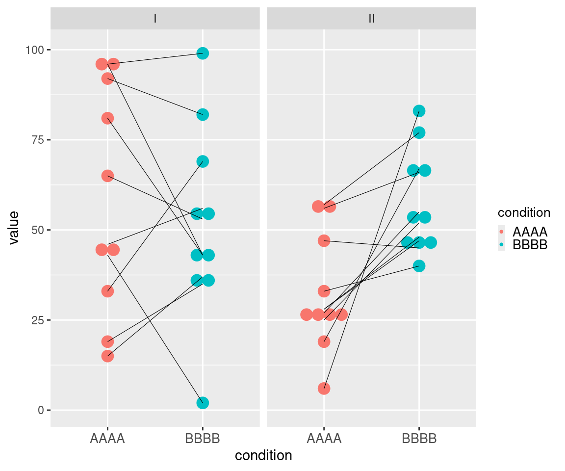
Table 6. Results of muMCW testing using an entry dataset with vertical layout
   contrast condition_a condition_b     N    test_type  BI_type
     <char>      <char>      <char> <int>       <char>   <char>
1:        I        AAAA        BBBB    10 approximated muMCW_BI
2:        I        AAAA        BBBB    10 approximated muMCW_BI
3:       II        AAAA        BBBB    10 approximated muMCW_BI
4:       II        AAAA        BBBB    10 approximated muMCW_BI
   condition_contrast observed_BI expected_by_chance_BI_N pupper plower
               <char>       <num>                   <int>  <num>  <num>
1:          AAAA-BBBB   0.2181818                     200  0.285  0.725
2:          BBBB-AAAA  -0.2181818                     200  0.725  0.285
3:          AAAA-BBBB  -0.9454545                     200  1.000  0.000
4:          BBBB-AAAA   0.9454545                     200  0.000  1.000
muMCW testing of multiple datasets organized horizontally
This example of muMCW testing entry dataset with a horizontal layout showcases data for six ideal tests (Table 7). It includes two types of informative columns to accommodate cases where users might want to perform multiple tests with a nested structure. The columns with the contrast prefix provide contextual information for groups of tests or rows, while the columns with the element prefix provide contextual information for each test or row. Each Contrast I row includes one set of matched-paired measures randomly selected from the same range (Figure 4). Each Contrast II row includes one set of matched-paired measures randomly selected from two different ranges, with the measures for the second condition in each matched-pair being generally higher than measures from the first condition in each matched-pair (Figure 4). The results of these muMCW tests align with the intended structure of the entry datasets (Table 8).
Table 7. muMCW testing entry dataset with horizontal layout
   contrast contrast_trait element_ID element_chr element_start element_end
     <char>         <char>     <char>       <int>         <int>       <int>
1:        I        trait_a         x1           1          1000        2000
2:        I        trait_a         x2           1          5000        5500
3:        I        trait_a         x3           1         90000      100000
4:       II        trait_b         x1           1          1000        2000
5:       II        trait_b         x2           1          5000        5500
6:       II        trait_b         x3           1         90000      100000
   condition_a condition_b   a.1   a.2   a.3   a.4   a.5   b.1   b.2   b.3
        <char>      <char> <int> <int> <int> <int> <int> <int> <int> <int>
1:        AAAA        BBBB    91    56    65    63    23    17    57    NA
2:        AAAA        BBBB    96    45    42    29    12    25    36    28
3:        AAAA        BBBB    77    98    31    93    34    34    97    77
4:        AAAA        BBBB    54    23    59    28    52    90    92    91
5:        AAAA        BBBB    37     5    18    26    11    48    84    62
6:        AAAA        BBBB    28    35    43    13     6    60    71    77
     b.4   b.5
   <int> <int>
1:    39    30
2:    79    82
3:    53    11
4:    50    68
5:    86    53
6:    89    97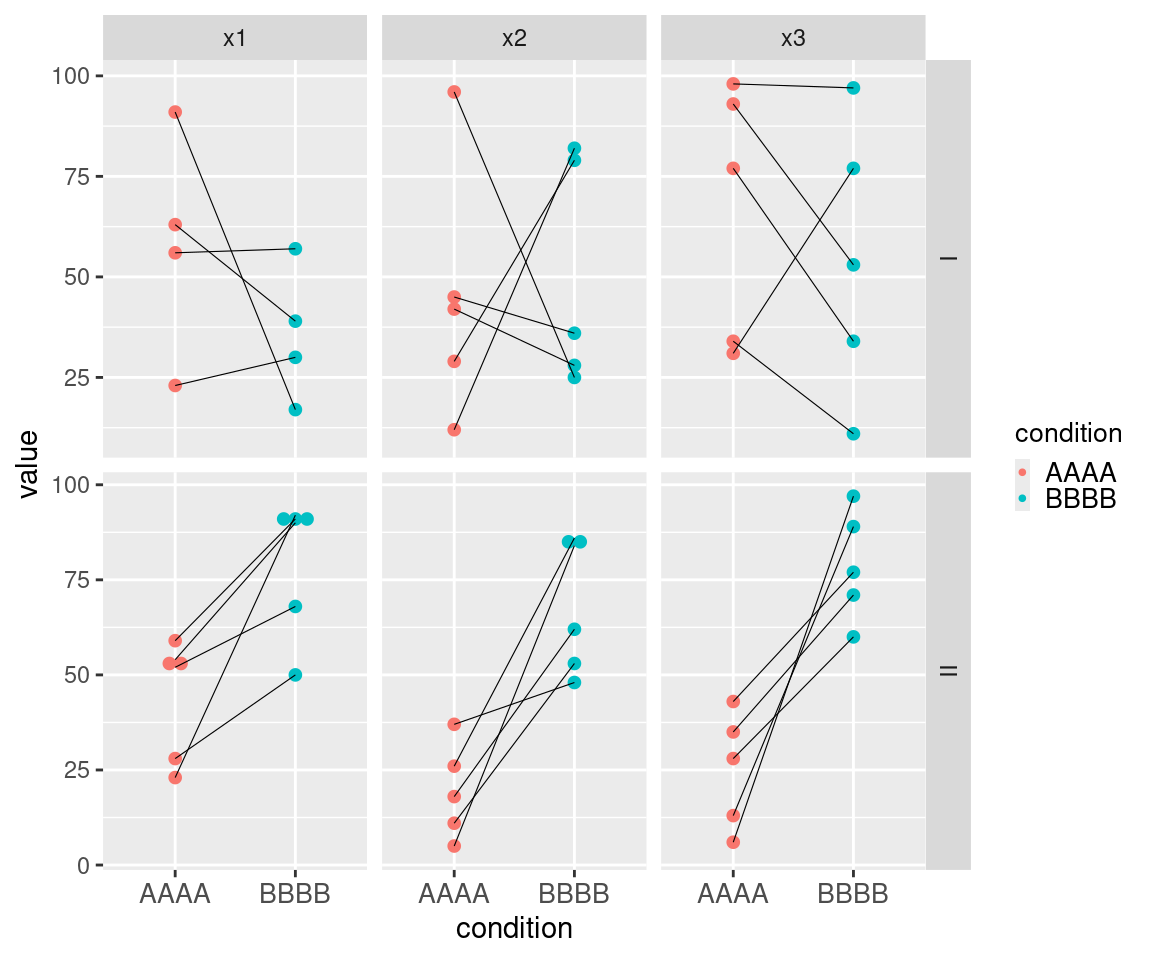
Table 8. Results of muMCW testing using an entry dataset with horizontal layout
    contrast contrast_trait element_ID element_chr element_start element_end
      <char>         <char>     <char>       <int>         <int>       <int>
 1:        I        trait_a         x1           1          1000        2000
 2:        I        trait_a         x1           1          1000        2000
 3:        I        trait_a         x2           1          5000        5500
 4:        I        trait_a         x2           1          5000        5500
 5:        I        trait_a         x3           1         90000      100000
 6:        I        trait_a         x3           1         90000      100000
 7:       II        trait_b         x1           1          1000        2000
 8:       II        trait_b         x1           1          1000        2000
 9:       II        trait_b         x2           1          5000        5500
10:       II        trait_b         x2           1          5000        5500
11:       II        trait_b         x3           1         90000      100000
12:       II        trait_b         x3           1         90000      100000
    condition_a condition_b     N    test_type  BI_type condition_contrast
         <char>      <char> <int>       <char>   <char>             <char>
 1:        AAAA        BBBB     4        exact muMCW_BI          AAAA-BBBB
 2:        AAAA        BBBB     4        exact muMCW_BI          BBBB-AAAA
 3:        AAAA        BBBB     5 approximated muMCW_BI          AAAA-BBBB
 4:        AAAA        BBBB     5 approximated muMCW_BI          BBBB-AAAA
 5:        AAAA        BBBB     5 approximated muMCW_BI          AAAA-BBBB
 6:        AAAA        BBBB     5 approximated muMCW_BI          BBBB-AAAA
 7:        AAAA        BBBB     5 approximated muMCW_BI          AAAA-BBBB
 8:        AAAA        BBBB     5 approximated muMCW_BI          BBBB-AAAA
 9:        AAAA        BBBB     5 approximated muMCW_BI          AAAA-BBBB
10:        AAAA        BBBB     5 approximated muMCW_BI          BBBB-AAAA
11:        AAAA        BBBB     5 approximated muMCW_BI          AAAA-BBBB
12:        AAAA        BBBB     5 approximated muMCW_BI          BBBB-AAAA
    observed_BI expected_by_chance_BI_N    pupper    plower
          <num>                   <int>     <num>     <num>
 1:  0.40000000                     105 0.7142857 0.6380952
 2: -0.40000000                     105 0.6380952 0.7142857
 3:  0.06666667                     200 0.4650000 0.6300000
 4: -0.06666667                     200 0.6300000 0.4650000
 5:  0.33333333                     200 0.3050000 0.7700000
 6: -0.33333333                     200 0.7700000 0.3050000
 7: -1.00000000                     200 1.0000000 0.0500000
 8:  1.00000000                     200 0.0500000 1.0000000
 9: -1.00000000                     200 1.0000000 0.0650000
10:  1.00000000                     200 0.0650000 1.0000000
11: -1.00000000                     200 1.0000000 0.0250000
12:  1.00000000                     200 0.0250000 1.0000000
4.3 matched-measures bivariate MCW (mbMCW) test
Introduction
The mbMCW test assesses whether two sets of inherently matched-paired measures are significantly differentially biased in the same direction. For instance, mbMCW tests can be used to analyze bodyweights or transcript abundances determined at two different timepoints for two sets of mice that have been exposed to different conditions.
mbMCW testing entry dataset formatting
When executing the mbMCWtest function, users must provide the path to a local CSV file named X_mbMCWtest_data.csv, where X serves as a user-defined identifier. X_mbMCWtest_data.csv can be structured in two distinct formats:
-
Vertical layout: This format allows appending datasets with varying structures, such as different numbers of matched-pairs per set or between each appended test. Vertical entry datasets should include the following columns:
- Columns matched_condition_a and matched_condition_b uniquely identify the two conditions under which matched-paired measure were collected.
- Column unmatched_condition uniquely identifies the two sets of matched-paired measures under analysis.
- Columns value_a and value_b contain the actual measures under analysis.
- As many informative columns as needed by users to contextualize the results of each test. The names of these columns should not contain the terms condition or value. While these columns are optional when running a single test, at least one column is required when running multiple tests simultaneously. All rows for each individual test must contain the same information in these columns.
-
Horizontal layout: This format allows appending datasets with similar structures, such as the same number of matched-paired measures collected for two conditions. Horizontal entry datasets should include the following columns:
- Columns matched_condition_a and matched_condition_b uniquely identify the two conditions under which matched-paired measure were collected.
- Columns unmatched_condition_x and unmatched_condition_y uniquely identify the two different sets of matched-paired measures under analysis.
- Columns x.a.i, y.a.i, x.b.i and y.b.i, where i represents integers to differentiate each specific matched-pair of measures, contain the actual measures under analysis.
- As many informative columns as needed by users to contextualize the results of each test. The name of these columns should not contain the term condition or have the same structure as the x.a.i, y.a.i, x.b.i and y.b.i columns. While these columns are optional when running a single test, at least one column is required when running multiple tests simultaneously.
mbMCW testing process
The function mbMCWtest eliminates any matched-paired measures with at least one missing value (NA) before proceeding with the following steps.
-
To estimate the differential bias between the two sets of matched-paired measures in the dataset, the function mbMCWtest perfoms the following tasks:
- For each matched-paired measure, it subtracts the values for the two possible matched condition contrasts (e.g., a-b and b-a).
- For each matched condition contrast, it ranks the absolute values of non-zero differences from lowest to highest. Measure pair differences with a value of 0 are assigned a 0 rank. If multiple measure pair differences have the same absolute value, all tied measure pair differences are assigned the lowest rank possible.
- It assigns each measure pair rank a sign based on the sign of its corresponding measure pair difference.
- For each set of matched-paired measures (e.g., x and y), it sums the signed ranks for each matched condition contrast (e.g., a-b and b-a).
- For each set of matched-paired measures (e.g., x and y) and each matched condition contrast (e.g., a-b and b-a), it calculates one mbMCW_BI. This value is obtained by dividing each sum of signed ranks by the maximum number this sum could have if the corresponding measure pairs had the highest possible positive ranks. Consequently, mbMCW_BI ranges between 1 when all the values for matched-pair measure differences in the set under analysis have the highest positive values, and -1 when all the values for matched-pair measure differences in the set under analysis have the lowest negative values.
-
To assess the significance of the mbMCW_BIs obtained from the user-provided dataset (observed mbMCW_BIs), the function mbMCWtest perfoms the following tasks:
-
It generates a collection of expected-by-chance mbMCW_BIs. These expected values are obtained by rearranging the matched-pair measures between the two sets multiple times. The user-provided parameter max_rearrangements determines the two paths the function mbMCWtest can follow to generate the collection of expected-by-chance mbMCW_BIs:
- mbMCW exact testing: If the number of distinct matched-paired measure rearrangements that can alter their initial set distribution is less than max_rearrangements, the function mbMCWtest calculates mbMCW_BIs for all possible data rearrangements.
- mbMCW approximated testing: If the number of distinct matched-paired measure rearrangements that can alter their initial set distribution is greater than max_rearrangements, the function mbMCWtest performs N = max_rearrangements random measure rearrangements to calculate the collection of expected-by-chance mbMCW_BIs.
It calculates Pupper and Plower values as the fraction of expected-by-chance mbMCW_BIs that are higher or equal to and lower or equal to the observed mbMCW_BIs, respectively.
-
mbMCW testing results
The mbMCWtest function reports to the console the total number of tests it will execute, and their exact and approximated counts. It also creates a CSV file named X_mbMCWtest_results.csv, where X is a user-defined identifier for the entry dataset CSV file. The X_mbMCWtest_results.csv file contains four rows for each mbMCWtest, with mbMCW_BIs calculated for each possible contrast between matched and unmatched measures (e.g., a-b, b-a, x-y and y-x).
The X_mbMCWtest_results.csv file includes the following columns:
- User-provided informative columns to contextualize the results of each test.
- Columns matched_condition_a and matched_condition_b indicate the conditions for which matched-paired measures were provided.
- Columns unmatched_condition_x and unmatched_condition_y indicate the two sets of matched-pairs measures.
- Columns N, N_x and N_y indicate the total number of matched-paired measures, and their distribution between the two unmatched sets after removing any matched-pair with missing values (NAs).
- Column test_type distinguishes between exact and approximated tests.
- Column BI_type indicates mbMCW_BI.
- Column matched_condition_contrast and unmatched_condition_contrast indicate the matched and unmatched condition contrast for each row of results.
- Column observed_BI contains the value of mbMCW_BIs obtained from analyzing the user-provided dataset.
- Column expected_by_chance_BI_N indicates the number of data rearrangements used to calculate the expected-by-chance mbMCW_BIs. This value corresponds to the lowest number between all possible measure rearrangements and the parameter max_rearrangements.
- Columns pupper and plower represent the Pupper and Plower values, respectively. They denote the fraction of expected-by-chance mbMCW_BIs with values higher or equal to and lower or equal to the observed mbMCW_BIs, respectively.
Examples
mbMCW testing of multiple datasets organized vertically
This example of mbMCW testing entry dataset with a vertical layout showcases data for two ideal tests (Table 9). The Contrast I test includes data for two sets of matched-paired measures randomly selected from the same range (Figure 5). The Contrast II test includes data for two sets of matched-paired measures. For the first set, matched-pair measures were randomly selected from the same range. For the second set, matched-pair measures were randomly selected from two different ranges, with the measures corresponding to the second condition of each matched-pair being generally higher than the measures corresponding to the first condition of each matched-pair (Figure 5). The results of these mbMCW tests align with the intended structure of the entry datasets (Table 10).
Table 9. mbMCW testing entry dataset with vertical layout
    contrast matched_condition_a matched_condition_b unmatched_condition
      <char>              <char>              <char>              <char>
 1:        I                AAAA                BBBB                XXXX
 2:        I                AAAA                BBBB                XXXX
 3:        I                AAAA                BBBB                XXXX
 4:        I                AAAA                BBBB                XXXX
 5:        I                AAAA                BBBB                XXXX
 6:        I                AAAA                BBBB                YYYY
 7:        I                AAAA                BBBB                YYYY
 8:        I                AAAA                BBBB                YYYY
 9:        I                AAAA                BBBB                YYYY
10:        I                AAAA                BBBB                YYYY
11:       II                AAAA                BBBB                XXXX
12:       II                AAAA                BBBB                XXXX
13:       II                AAAA                BBBB                XXXX
14:       II                AAAA                BBBB                XXXX
15:       II                AAAA                BBBB                XXXX
16:       II                AAAA                BBBB                YYYY
17:       II                AAAA                BBBB                YYYY
18:       II                AAAA                BBBB                YYYY
19:       II                AAAA                BBBB                YYYY
20:       II                AAAA                BBBB                YYYY
    contrast matched_condition_a matched_condition_b unmatched_condition
    value_a value_b
      <int>   <int>
 1:       6      37
 2:      25      18
 3:      13      27
 4:      48      16
 5:      44      70
 6:      30      19
 7:       9      24
 8:      16      47
 9:      47      33
10:      14      23
11:      13      47
12:      14      41
13:      42      13
14:      40      38
15:      47      11
16:      36      70
17:      38      64
18:      31      60
19:      33      67
20:      25      69
    value_a value_b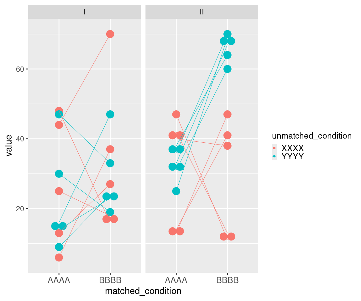
Table 10. Results of mbMCW testing using an entry dataset with vertical layout
   contrast matched_condition_a matched_condition_b unmatched_condition_x
     <char>              <char>              <char>                <char>
1:        I                AAAA                BBBB                  XXXX
2:        I                AAAA                BBBB                  XXXX
3:        I                AAAA                BBBB                  XXXX
4:        I                AAAA                BBBB                  XXXX
5:       II                AAAA                BBBB                  XXXX
6:       II                AAAA                BBBB                  XXXX
7:       II                AAAA                BBBB                  XXXX
8:       II                AAAA                BBBB                  XXXX
   unmatched_condition_y     N   N_x   N_y    test_type  BI_type
                  <char> <int> <int> <int>       <char>   <char>
1:                  YYYY    10     5     5 approximated mbMCW_BI
2:                  YYYY    10     5     5 approximated mbMCW_BI
3:                  YYYY    10     5     5 approximated mbMCW_BI
4:                  YYYY    10     5     5 approximated mbMCW_BI
5:                  YYYY    10     5     5 approximated mbMCW_BI
6:                  YYYY    10     5     5 approximated mbMCW_BI
7:                  YYYY    10     5     5 approximated mbMCW_BI
8:                  YYYY    10     5     5 approximated mbMCW_BI
   matched_condition_contrast unmatched_condition_contrast observed_BI
                       <char>                       <char>       <num>
1:                  AAAA-BBBB                    XXXX-YYYY  0.01886792
2:                  AAAA-BBBB                    YYYY-XXXX -0.01886792
3:                  BBBB-AAAA                    XXXX-YYYY -0.01886792
4:                  BBBB-AAAA                    YYYY-XXXX  0.01886792
5:                  AAAA-BBBB                    XXXX-YYYY  0.64705882
6:                  AAAA-BBBB                    YYYY-XXXX -0.64705882
7:                  BBBB-AAAA                    XXXX-YYYY -0.64705882
8:                  BBBB-AAAA                    YYYY-XXXX  0.64705882
   expected_by_chance_BI_N pupper plower
                     <int>  <num>  <num>
1:                     200  0.470  0.570
2:                     200  0.570  0.470
3:                     200  0.570  0.470
4:                     200  0.470  0.570
5:                     200  0.035  0.980
6:                     200  0.980  0.035
7:                     200  0.980  0.035
8:                     200  0.035  0.980
mbMCW testing of multiple datasets organized horizontally
This example of mbMCW testing entry dataset with a vertical layout showcases data for six tests (Table 11). It includes two types of informative columns to accommodate cases where users might want to perform multiple tests with a nested structure. The columns with the contrast prefix provide contextual information for groups of tests or rows, while the columns with the element prefix provide contextual information for each test or row. Each Contrast I row includes two sets of matched-paired measures randomly selected from the same range (Figure 6). Each Contrast II row includes two sets of matched-paired measures. For the first set, matched-pair measures were randomly selected from the same range. For the second set, matched-pair measures were randomly selected from two different ranges, with the measures corresponding to the second condition of each matched-pair being generally higher than the measures corresponding to the first condition of each matched-pair (Figure 6). The results of these mbMCW tests align with the intended structure of the entry datasets (Table 12).
Table 11. mbMCW testing entry dataset with horizontal layout
   contrast contrast_trait element_ID element_chr element_start element_end
     <char>         <char>     <char>       <int>         <int>       <int>
1:        I        trait_a         x1           1          1000        2000
2:        I        trait_a         x2           1          5000        5500
3:        I        trait_a         x3           1         90000      100000
4:       II        trait_b         x1           1          1000        2000
5:       II        trait_b         x2           1          5000        5500
6:       II        trait_b         x3           1         90000      100000
   matched_condition_a matched_condition_b unmatched_condition_x
                <char>              <char>                <char>
1:                AAAA                BBBB                  XXXX
2:                AAAA                BBBB                  XXXX
3:                AAAA                BBBB                  XXXX
4:                AAAA                BBBB                  XXXX
5:                AAAA                BBBB                  XXXX
6:                AAAA                BBBB                  XXXX
   unmatched_condition_y x.a.1 x.a.2 x.a.3 x.a.4 x.a.5 y.a.6 y.a.7 y.a.8 y.a.9
                  <char> <int> <int> <int> <int> <int> <int> <int> <int> <int>
1:                  YYYY     3    31    21     4    44    27    48    17    36
2:                  YYYY    20     7    30    27    40    34    34    17     7
3:                  YYYY    14    12    12    32    10    27    36    42    10
4:                  YYYY    12    16    35    36    38    36    49     6    22
5:                  YYYY     7    16    28    20    17    42    14    20    43
6:                  YYYY     5    30    17    46    22    47    13    32    20
   y.a.10 x.b.1 x.b.2 x.b.3 x.b.4 x.b.5 y.b.6 y.b.7 y.b.8 y.b.9 y.b.10
    <int> <int> <int> <int> <int> <int> <int> <int> <int> <int>  <int>
1:      7    42    70    17    30    17    18    36    20    36     48
2:     26    41    19     2     1    48    22    34     8    11      7
3:      5    25    27    23    13    14     2    43    35    21     23
4:      2    15    18    17    33    14    68    64    77    75     63
5:     29    26    31    25    48    16    54    61    51    68     68
6:     28    19    42    26    26    13    78    64    70    51     52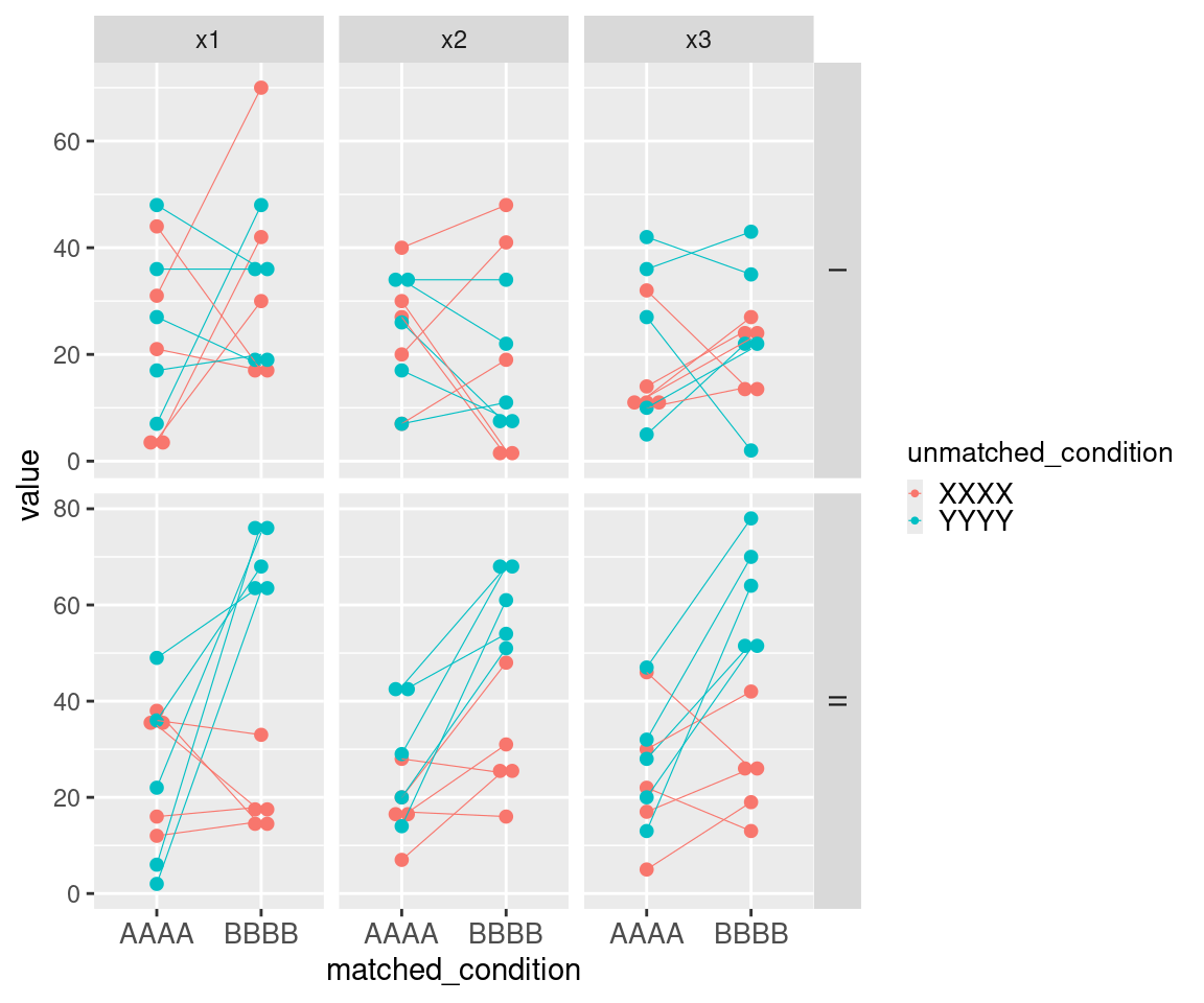
Table 12. Results of mbMCW testing using an entry dataset with horizontal layout
    contrast contrast_trait element_ID element_chr element_start element_end
      <char>         <char>     <char>       <int>         <int>       <int>
 1:        I        trait_a         x1           1          1000        2000
 2:        I        trait_a         x1           1          1000        2000
 3:        I        trait_a         x1           1          1000        2000
 4:        I        trait_a         x1           1          1000        2000
 5:        I        trait_a         x2           1          5000        5500
 6:        I        trait_a         x2           1          5000        5500
 7:        I        trait_a         x2           1          5000        5500
 8:        I        trait_a         x2           1          5000        5500
 9:        I        trait_a         x3           1         90000      100000
10:        I        trait_a         x3           1         90000      100000
11:        I        trait_a         x3           1         90000      100000
12:        I        trait_a         x3           1         90000      100000
13:       II        trait_b         x1           1          1000        2000
14:       II        trait_b         x1           1          1000        2000
15:       II        trait_b         x1           1          1000        2000
16:       II        trait_b         x1           1          1000        2000
17:       II        trait_b         x2           1          5000        5500
18:       II        trait_b         x2           1          5000        5500
19:       II        trait_b         x2           1          5000        5500
20:       II        trait_b         x2           1          5000        5500
21:       II        trait_b         x3           1         90000      100000
22:       II        trait_b         x3           1         90000      100000
23:       II        trait_b         x3           1         90000      100000
24:       II        trait_b         x3           1         90000      100000
    contrast contrast_trait element_ID element_chr element_start element_end
    matched_condition_a matched_condition_b unmatched_condition_x
                 <char>              <char>                <char>
 1:                AAAA                BBBB                  XXXX
 2:                AAAA                BBBB                  XXXX
 3:                AAAA                BBBB                  XXXX
 4:                AAAA                BBBB                  XXXX
 5:                AAAA                BBBB                  XXXX
 6:                AAAA                BBBB                  XXXX
 7:                AAAA                BBBB                  XXXX
 8:                AAAA                BBBB                  XXXX
 9:                AAAA                BBBB                  XXXX
10:                AAAA                BBBB                  XXXX
11:                AAAA                BBBB                  XXXX
12:                AAAA                BBBB                  XXXX
13:                AAAA                BBBB                  XXXX
14:                AAAA                BBBB                  XXXX
15:                AAAA                BBBB                  XXXX
16:                AAAA                BBBB                  XXXX
17:                AAAA                BBBB                  XXXX
18:                AAAA                BBBB                  XXXX
19:                AAAA                BBBB                  XXXX
20:                AAAA                BBBB                  XXXX
21:                AAAA                BBBB                  XXXX
22:                AAAA                BBBB                  XXXX
23:                AAAA                BBBB                  XXXX
24:                AAAA                BBBB                  XXXX
    matched_condition_a matched_condition_b unmatched_condition_x
    unmatched_condition_y     N   N_x   N_y    test_type  BI_type
                   <char> <int> <int> <int>       <char>   <char>
 1:                  YYYY    10     5     5 approximated mbMCW_BI
 2:                  YYYY    10     5     5 approximated mbMCW_BI
 3:                  YYYY    10     5     5 approximated mbMCW_BI
 4:                  YYYY    10     5     5 approximated mbMCW_BI
 5:                  YYYY    10     5     5 approximated mbMCW_BI
 6:                  YYYY    10     5     5 approximated mbMCW_BI
 7:                  YYYY    10     5     5 approximated mbMCW_BI
 8:                  YYYY    10     5     5 approximated mbMCW_BI
 9:                  YYYY    10     5     5 approximated mbMCW_BI
10:                  YYYY    10     5     5 approximated mbMCW_BI
11:                  YYYY    10     5     5 approximated mbMCW_BI
12:                  YYYY    10     5     5 approximated mbMCW_BI
13:                  YYYY    10     5     5 approximated mbMCW_BI
14:                  YYYY    10     5     5 approximated mbMCW_BI
15:                  YYYY    10     5     5 approximated mbMCW_BI
16:                  YYYY    10     5     5 approximated mbMCW_BI
17:                  YYYY    10     5     5 approximated mbMCW_BI
18:                  YYYY    10     5     5 approximated mbMCW_BI
19:                  YYYY    10     5     5 approximated mbMCW_BI
20:                  YYYY    10     5     5 approximated mbMCW_BI
21:                  YYYY    10     5     5 approximated mbMCW_BI
22:                  YYYY    10     5     5 approximated mbMCW_BI
23:                  YYYY    10     5     5 approximated mbMCW_BI
24:                  YYYY    10     5     5 approximated mbMCW_BI
    unmatched_condition_y     N   N_x   N_y    test_type  BI_type
    matched_condition_contrast unmatched_condition_contrast observed_BI
                        <char>                       <char>       <num>
 1:                  AAAA-BBBB                    XXXX-YYYY -0.18181818
 2:                  AAAA-BBBB                    YYYY-XXXX  0.18181818
 3:                  BBBB-AAAA                    XXXX-YYYY  0.18181818
 4:                  BBBB-AAAA                    YYYY-XXXX -0.18181818
 5:                  AAAA-BBBB                    XXXX-YYYY -0.18181818
 6:                  AAAA-BBBB                    YYYY-XXXX  0.18181818
 7:                  BBBB-AAAA                    XXXX-YYYY  0.18181818
 8:                  BBBB-AAAA                    YYYY-XXXX -0.18181818
 9:                  AAAA-BBBB                    XXXX-YYYY -0.09803922
10:                  AAAA-BBBB                    YYYY-XXXX  0.09803922
11:                  BBBB-AAAA                    XXXX-YYYY  0.09803922
12:                  BBBB-AAAA                    YYYY-XXXX -0.09803922
13:                  AAAA-BBBB                    XXXX-YYYY  0.88888889
14:                  AAAA-BBBB                    YYYY-XXXX -0.88888889
15:                  BBBB-AAAA                    XXXX-YYYY -0.88888889
16:                  BBBB-AAAA                    YYYY-XXXX  0.88888889
17:                  AAAA-BBBB                    XXXX-YYYY  0.41818182
18:                  AAAA-BBBB                    YYYY-XXXX -0.41818182
19:                  BBBB-AAAA                    XXXX-YYYY -0.41818182
20:                  BBBB-AAAA                    YYYY-XXXX  0.41818182
21:                  AAAA-BBBB                    XXXX-YYYY  0.69811321
22:                  AAAA-BBBB                    YYYY-XXXX -0.69811321
23:                  BBBB-AAAA                    XXXX-YYYY -0.69811321
24:                  BBBB-AAAA                    YYYY-XXXX  0.69811321
    matched_condition_contrast unmatched_condition_contrast observed_BI
    expected_by_chance_BI_N pupper plower
                      <int>  <num>  <num>
 1:                     200  0.660  0.375
 2:                     200  0.375  0.660
 3:                     200  0.375  0.660
 4:                     200  0.660  0.375
 5:                     200  0.720  0.315
 6:                     200  0.315  0.720
 7:                     200  0.315  0.720
 8:                     200  0.720  0.315
 9:                     200  0.630  0.425
10:                     200  0.425  0.630
11:                     200  0.425  0.630
12:                     200  0.630  0.425
13:                     200  0.000  1.000
14:                     200  1.000  0.000
15:                     200  1.000  0.000
16:                     200  0.000  1.000
17:                     200  0.035  0.975
18:                     200  0.975  0.035
19:                     200  0.975  0.035
20:                     200  0.035  0.975
21:                     200  0.005  1.000
22:                     200  1.000  0.005
23:                     200  1.000  0.005
24:                     200  0.005  1.000
    expected_by_chance_BI_N pupper plower
4.4 bias-measures MCW (bMCW) test
Introduction
The bMCW test is actually a combination of two tests that assess whether a set of measures of bias for a quantitative trait between two conditions or a subset of these bias measures are themselves significantly biased in the same direction. For instance, bMCW tests can be used to analyze bias indexes obtained using other MCW tests or fold change for transcript abundances spanning the entire transcriptome or only for genes located in specific genomic regions from two sets of mice exposed to different conditions.
bMCW testing entry dataset formatting
When executing the bMCWtest function, users must provide the path to a local CSV file named X_bMCWtest_data.csv, where X serves as a user-defined identifier. X_bMCWtest_data.csv should include the following columns:
- Column bias_value contains the value of the bias measure under analysis.
- Columns subset_x, where x represents the specific type of subset for each column, such as “chr” for chromosomes or “GO” for Gene Ontology. These columns are required if users intend to assess whether bias measures for certain subsets of elements in the dataset are significantly biased in the same direction. Columns subset_x can indicate whether an element belongs to a subset using either “YES” and “NO”, or specific subset names like “chr1” or “chrX”, or a combination of both, such as “chr1”, “chrX” and “NO”. The function bMCW test will transform the dataset to conduct independent analysis of each subset of elements marked as “YES” or with a specific subset name in each subset_x column.
- As many informative columns as needed by users to contextualize the results of each test. The names of these columns should not contain the terms bias_value or subset. While these columns are optional when running a single test, at least one column is required when running multiple tests simultaneously. All rows for each individual test must contain the same information in these columns.
- Users can specify columns with information relevant about each element or row using the column name structure element_x, where x indicates the specific information in each column (see example). However, element_x columns are not essential for bMCW testing and will not be included in the results file.
bMCW testing process
The function bMCWtest eliminates missing values (NAs) from the dataset before proceeding with the following steps.
-
To estimate the bias for all bias measures in the entire dataset or a subset of them, the function bMCWtest performs the following tasks:
- It ranks all bias measures with non-zero values from lowest to highest. Bias measures with a value of 0 are assigned a 0 rank. If multiple bias measures have the same absolute value, all tied bias measures are asssigned the lowest rank possible.
- It assigns each rank a sign based on the sign of its corresponding bias measure.
- It calculates a whole-set bias index (bMCW_wBI) by summing the signed ranks for all elements in the dataset and dividing it by the maximum number that sum could have if all bias measures were positive. Consequently, bMCW_wBI ranges between 1 when all bias measures are positive, and -1 when all bias measures are negative.
- It calculates a subset bias index (bMCW_sBI) for each subset of elements under analysis by summing the signed ranks for the elements in the subset and dividing it by the maximum number that sum could have if the elements in the subset had the highest possible positive bias measures. Consequently, bMCW_sBI ranges between 1 when the bias measures for the subset in question have the highest positive bias measures in the entire dataset, and -1 when the bias measures for the subset in question have the lowest negative bias measures in the entire dataset.
To assess the significance of the bMCW-wBIs and bMCW-sBIs obtained from the user-provided dataset (observed bMCW-wBIs and bMCW-sBIs), the function bMCWtest performs the following tasks,
- It generates a collection of expected-by-chance bMCW_wBIs by rearranging the signs of all signed ranks multiple times. The function *bMCWtest* also generates a collection of expected-by-chance bMCW_sBIs by rearranging the subset of elements multiple times. The user-provided parameter *max_rearrangements* determines the two paths that the function *bMCWtest* can follow to generate the collection of expected-by-chance bMCW_wBIs and bMCW_sBIs:

    - *bMCW exact testing*: If the number of distinct bias measure rearrangements that can alter their initial sign distribution or subset distribution is less than *max_rearrangements*, the function *bMCWtest* calculates bMCW_wBIs or bMCW_sBIs for all possible data rearrangements.
    - *bMCW approximated testing*: If the number of distinct bias measure rearrangements that can alter their initial sign distribution or subset distribution is greater than *max_rearrangements*, the function *bMCWtest* performs N = *max_rearrangements* random measure rearrangements to calculate the collection of expected-by-chance bMCW_wBIs or bMCW_sBIs.

- It calculates *P~upper~* and *P~lower~* values, as the fraction of expected-by-chance bMCW-wBIs and bMCW-sBIs that are higher or equal to and lower or equal to the observed bMCW-wBIs and bMCW-sBIs, respectively.
bMCW testing results
The bMCWtest function reports to the console the total number of tests it will execute, and their exact and approximated counts. It also creates a CSV file named X_bMCWtest_results.csv, where X is a user-defined identifier for the entry dataset CSV file. The X_bMCWtest_results.csv file contains one row for each bMCWtest to indicate the results of whole-set bMCW testing, and as many rows as necessary to indicate the results of subset bMCW testing. Rows for whole-set analyses will be at the top of X_bMCWtest_results.csv file.
The X_bMCWtest_results.csv file includes the following columns:
- User-provided informative columns to contextualize the results of each test.
- Column subset_type indicates whether the results in each row corresponds to whole-set tests or specific subset tests, such as “chr” for chromosomes or “GO” for Gene Ontology terms.
- Column tested_subset indicates the name of the subset under analysis. For whole-set tests, the tested_subset column indicates “none”. For subset tests, the tested_subset column indicates “YES” or the specific name of the subset under analysis, such as “chr1” or “chrX”.
- Columns N and n indicate the total number of elements in the whole set and those associated with the subset under analysis, respectively, after removing missing values (NAs). For whole-set tests, columns N and n have the same value.
- Column test_type distinguishes between exact and approximated tests.
- Column BI_type indicates whether results correspond to whole-set tests (bMCW_wBI) or to subset tests (bMCW_sBIs).
- Column observed_BI contains the value of bMCW_BIs obtained from analyzing the user-provided dataset.
- Column expected_by_chance_BI_N indicates the number of data rearrangements used to calculate the expected-by-chance bMCW_wBIs and bMCW_sBIs. This value corresponds to the lowest number between all possible measure rearrangements and the parameter max_rearrangements.
- Columns pupper and plower represent the Pupper and Plower values, respectively. They denote the fraction of expected-by-chance bMCW_wBIs or bMCW_sBIs with values higher or equal to and lower or equal to the observed bMCW_wBIs or bMCW_sBIs, respectively.
Examples
bMCW testing of multiple datasets
This example of bMCW testing entry dataset includes bias measures for three tests, each with ten elements distributed across four subsets: chr1, chr2, chrX and chrY (Table 13), In this example, the bias measures under study are uMCW_BIs, which range from 1 and -1. The Contrast I test includes bias measures randomly selected from the same range (Figure 7). The Contrast II test includes bias measures randomly selected from the same range, with most of them having positive values (Figure 7). The Contrast III includes bias measures randomly selected from the same range for three of the four subsets, while bias measures for the fourth subset are randomly selected with the largest positive values in the dataset (Figure 7). The results of these bMCW tests align with the intended structure of the entry datasets (Table 14).
Table 13. bMCW testing entry dataset
    contrast contrast_trait element_ID element_chr element_start element_end
      <char>         <char>     <char>      <char>         <int>       <int>
 1:        I        trait_a         x1        chr1          1000        2000
 2:        I        trait_a         x2        chr1          5000        5500
 3:        I        trait_a         x3        chr1         90000      100000
 4:        I        trait_a         x4        chr2           150         300
 5:        I        trait_a         x5        chr2          2545        7000
 6:        I        trait_a         x6        chr2         80000      100000
 7:        I        trait_a         x7        chrX          4000        7000
 8:        I        trait_a         x8        chrX          9000       10000
 9:        I        trait_a         x9        chrX         30000       31000
10:        I        trait_a        x10        chrY           800        1000
11:       II        trait_b         x1        chr1          1000        2000
12:       II        trait_b         x2        chr1          5000        5500
13:       II        trait_b         x3        chr1         90000      100000
14:       II        trait_b         x4        chr2           150         300
15:       II        trait_b         x5        chr2          2545        7000
16:       II        trait_b         x6        chr2         80000      100000
17:       II        trait_b         x7        chrX          4000        7000
18:       II        trait_b         x8        chrX          9000       10000
19:       II        trait_b         x9        chrX         30000       31000
20:       II        trait_b        x10        chrY           800        1000
21:      III        trait_c         x1        chr1          1000        2000
22:      III        trait_c         x2        chr1          5000        5500
23:      III        trait_c         x3        chr1         90000      100000
24:      III        trait_c         x4        chr2           150         300
25:      III        trait_c         x5        chr2          2545        7000
26:      III        trait_c         x6        chr2         80000      100000
27:      III        trait_c         x7        chrX          4000        7000
28:      III        trait_c         x8        chrX          9000       10000
29:      III        trait_c         x9        chrX         30000       31000
30:      III        trait_c        x10        chrY           800        1000
    contrast contrast_trait element_ID element_chr element_start element_end
    subset_chr bias_measure condition_contrast  bias_value
        <char>       <char>             <char>       <num>
 1:       chr1      uMCW_BI          AAAA-BBBB  0.59883185
 2:       chr1      uMCW_BI          AAAA-BBBB -0.37376010
 3:       chr1      uMCW_BI          AAAA-BBBB  0.75433521
 4:       chr2      uMCW_BI          AAAA-BBBB -0.36807420
 5:       chr2      uMCW_BI          AAAA-BBBB -0.97818020
 6:       chr2      uMCW_BI          AAAA-BBBB  0.59299509
 7:       chrX      uMCW_BI          AAAA-BBBB -0.58644011
 8:       chrX      uMCW_BI          AAAA-BBBB -0.36797886
 9:       chrX      uMCW_BI          AAAA-BBBB -0.63406711
10:       chrY      uMCW_BI          AAAA-BBBB  0.17762437
11:       chr1      uMCW_BI          AAAA-BBBB -0.03649558
12:       chr1      uMCW_BI          AAAA-BBBB  0.74867686
13:       chr1      uMCW_BI          AAAA-BBBB  0.81900144
14:       chr2      uMCW_BI          AAAA-BBBB  0.95044745
15:       chr2      uMCW_BI          AAAA-BBBB  0.87731860
16:       chr2      uMCW_BI          AAAA-BBBB  0.30838414
17:       chrX      uMCW_BI          AAAA-BBBB  0.44241725
18:       chrX      uMCW_BI          AAAA-BBBB  0.83965786
19:       chrX      uMCW_BI          AAAA-BBBB  0.65278713
20:       chrY      uMCW_BI          AAAA-BBBB -0.41912458
21:       chr1      uMCW_BI          AAAA-BBBB  0.42249472
22:       chr1      uMCW_BI          AAAA-BBBB  0.69599878
23:       chr1      uMCW_BI          AAAA-BBBB  0.59133980
24:       chr2      uMCW_BI          AAAA-BBBB -0.04787103
25:       chr2      uMCW_BI          AAAA-BBBB  0.01716967
26:       chr2      uMCW_BI          AAAA-BBBB  0.09079163
27:       chrX      uMCW_BI          AAAA-BBBB -0.07600623
28:       chrX      uMCW_BI          AAAA-BBBB -0.09808774
29:       chrX      uMCW_BI          AAAA-BBBB -0.02192925
30:       chrY      uMCW_BI          AAAA-BBBB -0.08190336
    subset_chr bias_measure condition_contrast  bias_value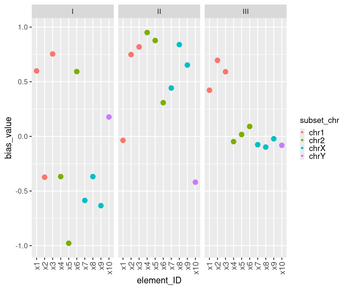
Table 14. bMCW testing results
    contrast contrast_trait bias_measure condition_contrast subset_type
      <char>         <char>       <char>             <char>      <char>
 1:        I        trait_a      uMCW_BI          AAAA-BBBB    wholeset
 2:       II        trait_b      uMCW_BI          AAAA-BBBB    wholeset
 3:      III        trait_c      uMCW_BI          AAAA-BBBB    wholeset
 4:        I        trait_a      uMCW_BI          AAAA-BBBB  subset_chr
 5:        I        trait_a      uMCW_BI          AAAA-BBBB  subset_chr
 6:        I        trait_a      uMCW_BI          AAAA-BBBB  subset_chr
 7:        I        trait_a      uMCW_BI          AAAA-BBBB  subset_chr
 8:       II        trait_b      uMCW_BI          AAAA-BBBB  subset_chr
 9:       II        trait_b      uMCW_BI          AAAA-BBBB  subset_chr
10:       II        trait_b      uMCW_BI          AAAA-BBBB  subset_chr
11:       II        trait_b      uMCW_BI          AAAA-BBBB  subset_chr
12:      III        trait_c      uMCW_BI          AAAA-BBBB  subset_chr
13:      III        trait_c      uMCW_BI          AAAA-BBBB  subset_chr
14:      III        trait_c      uMCW_BI          AAAA-BBBB  subset_chr
15:      III        trait_c      uMCW_BI          AAAA-BBBB  subset_chr
    tested_subset     N     n    test_type  BI_type observed_BI
           <char> <int> <int>       <char>   <char>       <num>
 1:          none    10    10 approximated bMCW_wBI  -0.1636364
 2:          none    10    10 approximated bMCW_wBI   0.8545455
 3:          none    10    10 approximated bMCW_wBI   0.2363636
 4:          chr1    10     3        exact bMCW_sBI   0.4444444
 5:          chr2    10     3        exact bMCW_sBI  -0.2592593
 6:          chrX    10     3        exact bMCW_sBI  -0.5555556
 7:          chrY    10     1        exact bMCW_sBI   0.1000000
 8:          chr1    10     3        exact bMCW_sBI   0.4444444
 9:          chr2    10     3        exact bMCW_sBI   0.7777778
10:          chrX    10     3        exact bMCW_sBI   0.6296296
11:          chrY    10     1        exact bMCW_sBI  -0.3000000
12:          chr1    10     3        exact bMCW_sBI   1.0000000
13:          chr2    10     3        exact bMCW_sBI   0.1481481
14:          chrX    10     3        exact bMCW_sBI  -0.4814815
15:          chrY    10     1        exact bMCW_sBI  -0.5000000
    expected_by_chance_BI_N      pupper     plower
                      <int>       <num>      <num>
 1:                     200 0.435000000 0.64500000
 2:                     200 0.050000000 0.96500000
 3:                     200 0.090000000 0.92500000
 4:                     120 0.075000000 0.94166667
 5:                     120 0.700000000 0.33333333
 6:                     120 0.900000000 0.12500000
 7:                      10 0.400000000 0.70000000
 8:                     120 0.658333333 0.40000000
 9:                     120 0.175000000 0.87500000
10:                     120 0.366666667 0.68333333
11:                      10 1.000000000 0.10000000
12:                     120 0.008333333 1.00000000
13:                     120 0.483333333 0.55833333
14:                     120 0.966666667 0.04166667
15:                      10 0.900000000 0.20000000